5. Data Processing and Analysis
After questionnaire development, pretesting the instrument and designing the sample, fieldwork – or the actual gathering of the required data – must be undertaken. However, we will not be discussing the complex and expensive tasks associated with fieldwork as part of this course.
Once the results start to come back from the field, the information needs to be prepared for input in order to be tabulated and analyzed. Before the questionnaires are given to someone for data-entry, they must be edited and coded. There should be no ambiguity as to what the respondent meant and what should be entered. This may sound simple, but what do you do in the following case:

So is it their first trip or not? And what do you instruct the data-entry person to do? In spite of clear instructions, this type of confusing response is not as rare as we might think, particularly in self-administered surveys.
If the questionnaire was not pre-coded, this will be done at the same time as the editing by the researcher. Coding involves assigning a label to each question or variable (as in "q15" or "1sttrip") and a number or value to each response category (for instance 1 for "yes" and 2 for "no"). Sometimes, people will write in a response such as "can’t remember" or "unsure", and the editor must decide on what to do. This could either be ignored or a new code and/or value could be added. All of these decisions as well as the questions and their codes are summarized in a "codebook" for future reference. Pamela Narins and J. Walter Thomson of SPSS have prepared some basic guidelines for preparing for data entry, that you should be sure to read.
Even in a structured questionnaire, you may have one or two open-ended questions, which do not lend themselves to coding. This type of question needs to be content analyzed and hopefully grouped into categories that are meaningful. At this point, they can be either tabulated manually or codes can be established for them.
Once the data has been input into the computer, usually with the assistance of a statistical package such as SPSS, it needs to be ‘cleaned’. This is the process of ensuring that the data entry was correctly executed and correcting any errors. There are a number of ways for checking for accuracy:
- Double entry: the data is entered twice and any discrepancies are verified against the original questionnaire;
- Running frequency distributions and scanning for errors in values based on the original questionnaire (if only four responses are possible, there should be no value "5", for instance); and
- Data listing refers to the printout of the values for all cases that have been entered and verifying a random sample of cases against the original questionnaires.
The objective is of course to achieve more accurate analysis through data cleaning, as explained by Pamela Narins and J. Walter Thompson of SPSS.
The data is now ready for tabulation and statistical analysis. This means that we want to do one or more of the following:
- Describe the background of the respondents, usually using their demographic information;
- Describe the responses made to each of the questions;
- Compare the behaviour of various demographic categories to one another to see if the differences are meaningful or simply due to chance;
- Determine if there is a relationship between two characteristics as described; and
- Predict whether one or more characteristic can explain the difference that occurs in another.
In order to describe the background of the respondents, we need to add up the number of responses and report them as percentages in what is called a frequency distribution (e.g. "Women accounted for 54% of visitors."). Similarly, when we describe the responses made to each of the questions; this information can be provided as a frequency, but with added information about the "typical" response or "average", which is also referred as measure of central tendency (e.g. "On average, visitors returned 13 times in the past five years".)
In order to compare the behaviour of various demographic categories to one another to see if the differences are meaningful or simply due to chance, we are really determining the statistical significance by tabulating two or more variables against each other in a cross-tabulation (e.g. "There is clear evidence of a relationship between gender and attendance at cultural venues. Attendance by women was statistically higher than men’s".).
If we wish to determine if there is a relationship between two characteristics as described; for instance the importance of predictable weather on a vacation and the ranking of destination types, then we are calculating the correlation. And finally, when trying to predict whether one or more characteristic can explain the difference that occurs in another, we might answer a question such as "Are gender, education and/or income levels linked to the number of times a person attends a cultural venue?
Frequency Distribution
The tally or frequency count is the calculation of how many people fit into a certain category or the number of times a characteristic occurs. This calculation is expressed by both the absolute (actual number) and relative (percentage) totals.
The example below is a typical output by the statistical software package SPSS. It provides us with the following information by column, starting from left to right:
- Column 1: the "valid" or useable information obtained as well as how many respondents did not provide the information and the total of the two.
- Column 2: the names of the "values" or choices people had in answering the particular question (in this case "high school or less", "some college/university", "graduated college/university or more") the total of these values and the reason why the information is missing. "System" refers to an answer that was not provided. Other choices might be "don’t know", "not applicable" or "can’t remember", which we might wish to discount in our total.
- Column 3: "frequency" refers to the actual number of respondents. As we can see, 95 people had a high school or less education, 263 had some college or university and 790 had graduated college/university or more, for a total of 1148. 60 people did not provide an answer, for a total of 1208 respondents in the survey. (This number should almost always be the same for all questions analyzed, although the number of "missing" could vary widely.)
- Column 4: "percent" is the calculation in percentage terms of the relative weight of each of the categories, but taking the full number of 1208 respondents in the survey as the base. Since we are rarely interested in including the ‘missing’ category as part of our analysis, this percentage is rarely used.
- Column 5: "valid percent" is the calculation in percentage terms of the relative weight of each of the "valid" categories only. Hence it uses only those who responded to the question, or 1148, for the calculation. It is this column that is normally used for all data analysis.
- Column 6: when adding the valid percent column together row by row, you get the corresponding "cumulative percentage". In this example, "high school or less" (8.3) plus "some college/university (22.9) equals the cumulative percentage of 31.2 (8.3 + 22.9). When you add the third category of "graduated college/university or more" (68.8) to the first two, you will reach 100. This column is particularly useful when dealing with many response categories and trying to determine where the median falls.
Highest level of education
|
Frequency |
Percent |
Valid Percent |
Cumulative Percent |
||
| Valid | high school or less |
95 |
7.9 |
8.3 |
8.3 |
| some college/university |
263 |
21.8 |
22.9 |
31.2 |
|
| graduated college/ university or more |
790 |
65.4 |
68.8 |
100.0 |
|
| Total |
1148 |
95.0 |
100.0 |
||
| Missing | System |
60 |
5.0 |
||
|
Total |
1208 |
100.0 |
There are two common ways of graphically representing this information. The first is in the form of a pie chart (Figure 1), which takes the percentage column and represents it in the form of pieces of pie based on the percentage for each category. You will notice that any graph should be given a number (e.g. Figure 1), a title (e.g. Highest level of education) and the total number of respondents that participated in the survey (n=1208). Pie charts should be used to only to express percentages or proportions, such as marketshare.


Another way to graph the information is through a bar chart (Figure 2). In this case, we used a simple bar graph. Notice also that you are able to eliminate the missing category from the graph and therefore base the analysis on the 1148 respondents who answered this particular question. This is preferable to using a pie chart in the SPSS program, which will not allow you to eliminate the missing cases.
Line charts are used when plotting the chance in a variable over time. For example, if this same study had been undertaken every two years for the past ten, you might want to present this information graphically by showing the evolution in each education level with a line.
Calculation of Central Tendencies
Measures of central tendency describe the location of the center of a frequency distribution. There are three different measures of central tendency: the mode, median and mean.
The mode is simply the value of the observation that occurs most frequently. It is useful when you want the prevailing or most popular characteristic or quality. In a survey of adults aged 18 or older, the question "What is your age?" was answered as follows:
What is your age?
| Frequency | Percent | Valid Percent | Cumulative Percent | ||
| Valid | 18 | 17 | 1.1 | 1.1 | 1.1 |
| 19 | 14 | 0.9 | 0.9 | 2.1 | |
| 20 | 12 | 0.8 | 0.8 | 2.9 | |
| 21 | 21 | 1.4 | 1.4 | 4.3 | |
| 22 | 14 | 0.9 | 0.9 | 5.2 | |
| 23 | 24 | 1.6 | 1.6 | 6.8 | |
| 24 | 13 | 0.9 | 0.9 | 7.7 | |
| 25 | 25 | 1.7 | 1.7 | 9.3 | |
| 26 | 21 | 1.4 | 1.4 | 10.7 | |
| 27 | 23 | 1.5 | 1.5 | 12.3 | |
| 28 | 21 | 1.4 | 1.4 | 13.7 | |
| 29 | 20 | 1.3 | 1.3 | 15 | |
| 30 | 27 | 1.8 | 1.8 | 16.8 | |
| 31 | 20 | 1.3 | 1.3 | 18.1 | |
| 32 | 20 | 1.3 | 1.3 | 19.5 | |
| 33 | 24 | 1.6 | 1.6 | 21.1 | |
| 34 | 25 | 1.7 | 1.7 | 22.7 | |
| 35 | 27 | 1.8 | 1.8 | 24.5 | |
| 36 | 27 | 1.8 | 1.8 | 26.3 | |
| 37 | 19 | 1.3 | 1.3 | 27.6 | |
| 38 | 36 | 2.4 | 2.4 | 30 | |
| 39 | 32 | 2.1 | 2.1 | 32.1 | |
| 40 | 33 | 2.2 | 2.2 | 34.3 | |
| 41 | 31 | 2.1 | 2.1 | 36.4 | |
| 42 | 42 | 2.8 | 2.8 | 39.2 | |
| 43 | 32 | 2.1 | 2.1 | 41.3 | |
| 44 | 39 | 2.6 | 2.6 | 43.9 | |
| 45 | 34 | 2.3 | 2.3 | 46.2 | |
| 46 | 47 | 3.1 | 3.1 | 49.3 | |
| 47 | 30 | 2 | 2 | 51.3 | |
| 48 | 39 | 2.6 | 2.6 | 53.9 | |
| 49 | 33 | 2.2 | 2.2 | 56.1 | |
| 50 | 40 | 2.7 | 2.7 | 58.8 | |
| 51 | 27 | 1.8 | 1.8 | 60.6 | |
| 52 | 39 | 2.6 | 2.6 | 63.2 | |
| 53 | 31 | 2.1 | 2.1 | 65.3 | |
| 54 | 24 | 1.6 | 1.6 | 66.9 | |
| 55 | 38 | 2.5 | 2.5 | 69.4 | |
| 56 | 25 | 1.7 | 1.7 | 71.1 | |
| 57 | 22 | 1.5 | 1.5 | 72.5 | |
| 58 | 24 | 1.6 | 1.6 | 74.1 | |
| 59 | 21 | 1.4 | 1.4 | 75.5 | |
| 60 | 43 | 2.9 | 2.9 | 78.4 | |
| 61 | 29 | 1.9 | 1.9 | 80.3 | |
| 62 | 28 | 1.9 | 1.9 | 82.2 | |
| 63 | 25 | 1.7 | 1.7 | 83.9 | |
| 64 | 19 | 1.3 | 1.3 | 85.1 | |
| 65 | 39 | 2.6 | 2.6 | 87.7 | |
| 66 | 20 | 1.3 | 1.3 | 89.1 | |
| 67 | 14 | 0.9 | 0.9 | 90 | |
| 68 | 22 | 1.5 | 1.5 | 91.5 | |
| 69 | 25 | 1.7 | 1.7 | 93.1 | |
| 70 | 19 | 1.3 | 1.3 | 94.4 | |
| 71 | 9 | 0.6 | 0.6 | 95 | |
| 72 | 20 | 1.3 | 1.3 | 96.3 | |
| 73 | 8 | 0.5 | 0.5 | 96.9 | |
| 74 | 16 | 1.1 | 1.1 | 97.9 | |
| 75 | 10 | 0.7 | 0.7 | 98.6 | |
| 76 | 4 | 0.3 | 0.3 | 98.9 | |
| 77 | 4 | 0.3 | 0.3 | 99.1 | |
| 78 | 4 | 0.3 | 0.3 | 99.4 | |
| 79 | 1 | 0.1 | 0.1 | 99.5 | |
| 80 | 4 | 0.3 | 0.3 | 99.7 | |
| 81 | 1 | 0.1 | 0.1 | 99.8 | |
| 82 | 1 | 0.1 | 0.1 | 99.9 | |
| 84 | 1 | 0.1 | 0.1 | 99.9 | |
| 86 | 1 | 0.1 | 0.1 | 100 | |
| Total | 1500 | 100 | 100 |
Hence the mode is 46, since 47 respondents provided this answer, more than any other category. Since there is only one mode in this distribution, it is referred to as ‘unimodal’. If a distribution has two modes (or two values that have the same amount of responses that are also the highest), it is referred to as ‘bimodal’.
The median is the middle observation, where half the respondents have provided smaller values, and half larger ones. It is calculated by arranging all observations from lowest to highest score and counting to the middle value. In our example above, the median is 47. The cumulative percentage will tell you at a glance where the median falls. Since the median is not as sensitive as the mean to extreme values, it is used most commonly in cases where you are dealing with ‘outliers’ or extreme values in the distribution that would skew your data in some way. The median is also useful when dealing with ordinal data and you are most concerned with a typical score.
The mean is also known as the ‘arithmetic average’ and is symbolized by ‘X’. The formula for calculating the mean is ∑ X/n (The Greek letter sigma ∑ is the symbol for sum) This means that you total all responses (X) and then divide them by the total number of observations (n). In our example, you would have to multiply all the values (actual ages or ‘x’) by the number of respondents or frequencies (‘f’) for each (∑ x • f = X or. 18 • 17 + 19 • 14 + etc.) and then divide the total by the 1500 respondents who participated in the survey. The result is 47.04. Since the computer will follow the same steps, you must be sure that the values are real and not just codes for categories. For example, the computer would calculate a mean of 3.7367 for the same information as the frequency above but recoded into age categories, based on the assumption that the values under x are 1 to 6:
What is your age?
| Frequency | Percent | Valid Percent | Cumulative Percent | ||
| Valid | 18-24 years (1) | 115 | 7.7 | 7.7 | 7.7 |
| 25-34 years (2) | 226 | 15.1 | 15.1 | 22.7 | |
| 35-44 years (3) | 318 | 21.2 | 21.2 | 43.9 | |
| 45-54 years (4) | 344 | 22.9 | 22.9 | 66.9 | |
| 55-64 years (5) | 274 | 18.3 | 18.3 | 85.1 | |
| 65 years or more (6) | 223 | 14.9 | 14.9 | 100 | |
| Total | 1500 | 100 | 100 |
Another useful calculation is the range, the calculation of the spread of the numerical data. It is calculated by subtracting the lowest value (in our example 18) from the highest value (or 86) to give us a total of 68. This is particularly useful when dealing with rating scores, for instance, where you would like to determine how close people are in agreement or alternatively, how wide the discrepancies are.
Cross Tabulations
When you want to know how respondents answered on two or more questions at the same time, you will need to run a cross-tabulation. In order to do so, you must first determine which is your independent variable, and which your dependent variable, since the first is traditionally used as column headings and the latter are found in the row.
Independent variables explain or predict a response or an outcome, which is the dependent variable under study. As a basic rule, demographic information is usually considered independent, since characteristics such as gender, age, education etc. will normally determine the responses we make. If the variables being studied are not demographic, then the independent variable is determined by the study’s objectives. For instance, if the objective is to determine whether the level of satisfaction with the past holiday at a destination influences the likelihood of return, then level of satisfaction is our independent variable and the likelihood to return the dependent one.
This is the typical output of a simple cross-tabulation (of education levels and overall satisfaction with a holiday) as produced by SPSS, when we also ask that column percentage be calculated. Note that the title gives the two variables with the dependent one first separated by *. When producing this information in a table, we would reword it to read "Overall holiday satisfaction by highest level of education completed" ( see Table 1), removing all extraneous information and leaving it as a statement, not a question.
Overall satisfaction with your holiday * What is the highest level of education completed Crosstabulation
Obviously, you would not be able to use this table as is in a report. It requires ‘cleaning’. Your first consideration would be whether you want to keep all of the categories in your independent and dependent variable. This depends, of course, on what you are trying to illustrate and the responses in each cell. First of all, very few people have less than a high school degree, and we could therefore collapse the first two categories into ‘high school or less’. But that still leaves us with five categories or more detail than we would probably need. So we could collapse the categories ‘graduated from technical or vocational school’ and ‘some college/university’ into ‘some advanced education’ and the last two into ‘graduated from university or more’. Similarly, we notice that the level of satisfaction with the holiday is very high. Indeed, any rows with less than 5% of respondents in cells should be collapsed. At the very least we should only have one category ‘not at all or nor very satisfied’. This collapsing of categories is knows as recoding and is a way of changing existing variables or creating new variables based on existing data as explained by John Urbik, the Technical Marketing Specialist for SPSS.
The resultant cross-tabulation would look like this:
overall satisfaction with holiday * highest level of education Crosstabulation
| What is the highest level of education completed | Total | |||||||||
| Primary school (grade 1-7) | Some high school | Graduated from high school | Graduated from a technical or vocational school | Some college or university | Graduated from university | Graduated with an advanced degree | ||||
| Overall satisfaction with your holiday | Not at all satisfied | Count | 2 | 1 | 1 | 1 | 5 | |||
| % within What is the highest level of education completed | 0.60% | 0.40% | 0.50% | 1.10% | 0.40% | |||||
| Not very satisfied | Count | 2 | 6 | 8 | 8 | 2 | 1 | 2 | 29 | |
| % within What is the highest level of education completed | 6.70% | 1.80% | 3.00% | 4.00% | 1.40% | 0.40% | 2.20% | 2.20% | ||
| Somewhat satisfied | Count | 3 | 40 | 37 | 25 | 30 | 42 | 12 | 189 | |
| % within What is the highest level of education completed | 10.00% | 11.80% | 13.70% | 12.60% | 21.30% | 15.80% | 13.00% | 14.20% | ||
| Very satisfied | Count | 25 | 290 | 224 | 164 | 109 | 223 | 77 | 1112 | |
| % within What is the highest level of education completed | 83.30% | 85.80% | 83.00% | 82.80% | 77.30% | 83.80% | 83.70% | 83.30% | ||
| Total | Count | 30 | 338 | 270 | 198 | 141 | 266 | 92 | 1335 | |
| % within What is the highest level of education completed | 100.00% | 100.00% | 100.00% | 100.00% | 100.00% | 100.00% | 100.00% | 100.00% |
We can now proceed to present this information in a more pleasing table format by giving it the appropriate table number and title, indicating the total number of respondents who answered this question, and cleaning the table, as follows:
Table 1: Overall holiday satisfaction by highest level of education
n=1243
| Degree of Satisfaction | Level of education | ||
| High school or less | Some advanced education | Graduated university of more | |
| Not at all or not very |
10 2.7% |
18 3.8% |
3 .7% |
| Somewhat |
43 11.7% |
62 13.2% |
72 17.7% |
| Very |
315 85.6% |
388 82.9% |
332 81.6% |
| Total |
368 100% |
468 100% |
407 100% |
Graphically, we would follow very similar rules: the graph is numbered (Figure 1) with the same title and the number of respondents indicated; the independent variable identifies the columns since we want to compare the satisfaction level of each of the three education categories. It is the column percentage that is used for comparison purposes. The type of graph below is called a clustered bar chart.
Calculating the Chi-Square
The chi-square (pronounced ‘kai’) distribution is the most commonly used method of comparing proportions. Its symbolized by the Greek letter chi or χ2). This test makes it possible to determine whether the difference exists between two groups and their preference or likelihood of doing something is real or just a chance occurrence. In other words, it determines whether a relationship or association exists between being in one of the two groups and the behaviour or characteristic under study. If in a survey of 692 respondents we asked whether or not they are interested attending attractions and events that deal with history and heritage during their vacation, and we wanted to determine whether there is a difference in how men and women respond to this question, we could calculate a chi-square.
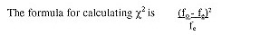
χ2 determines the differences between the observed (fo) and expected frequencies (fe). The observed frequencies are the actual survey results, whereas the expected frequencies refer to the hypothetical distribution based on the overall proportions between the two characteristics if the two groups are alike. For example, if we have the following survey results:
| Observed frequencies | |||
| History & Heritage | Men | Women | Total |
| Yes | 95 | 159 | 254 |
| No | 199 | 239 | 438 |
| Total | 294 | 398 | 692 |
Then we can calculate our expected frequencies (fe) based on the proportion of respondents who said ‘yes’ versus ‘no’. It can also be calculated for each cell by the row total with the column total divided by the grand total (e.g. 254 x 294 : 692 = 108).
| Expected frequencies | |||
| History & Heritage | Men | Women | Total |
| Yes | 108 | 146 | 254 |
| No | 186 | 252 | 438 |
| Total | 294 | 398 | 692 |
This second table, where no relationship exists between the interest in attending history and heritage attractions and events and gender, also represents the null hypothesis or Ho. (Therefore, if a study says that it "fails to reject the null hypothesis", it means that no relationship was found to exist between the variables under study.)
Hence, the calculation is as follows:
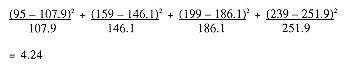
The critical value for a level of significance of .05 (or 95% level of confidence, the normal level in this type of research) is 3.841. This means that you are confident that 95% of the distribution falls below this critical value. Since our result is above this value, we can:
- Reject the null hypothesis that no difference exists between interest in attending historical attractions and events and gender (in other words, there is a difference between genders); and
- Conclude that the differences in the groups are statistically significant (or not due to chance)
You will not need to memorize all the critical values since computer programs such as SPSS will not only calculate the χ2 values for you, but will also give you the precise level of observed significance (known as p value), which in our case is .039. If this level of significance is above the standard .05 level of statistical significance, you are dealing with a statistically significant relationship.
Determining Correlation
A correlation is used to estimate the relationship between two characteristics. If we are dealing with two ordinal or one ordinal and one numerical (interval or ratio) characteristic, then the correct correlation to use is the Spearman rank correlation, named after the statistician, also known as rho or rs. Computer software programs such as SPSS will execute the tedious task of calculating Spearman’s rho very easily.
Correlations range from –1 to +1. At these extremes, the correlation between the two characteristics is perfect, although it is negative or inverse in the first instance. A perfect correlation is one where the two characteristics increase or decrease by the same amount. This is a linear relationship as illustrated below.
A correlation coefficient of 0 therefore refers to a situation where no relationship exists between the two characteristics. In other words, changes in one characteristic cannot be explained by the changes occurring in the second characteristic. A common way of interpreting the strength of a correlation is as follows:
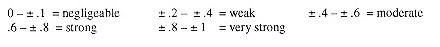
However, in most tourism and hospitality related research, corrections between ± .26 to ± .5 are generally considered to be quite high, with strong or very strong correlations rarely found.
The variation in one characteristic can be predicted if we know the value of correlation, since we can calculate the coefficient of determination or r2.
If we have a correlation of ±.5, then ±.52 = .25. We can therefore conclude that 25% of the variation in one characteristics can be predicted by the value of the second measure.
Let us take a look at an example to make these interpretations clearer. Let us assume we wish to determine whether pleasure travellers who are interested in staying in first class hotels are motivated because they wish to indulge in luxury or because of some other motivation, such as the identification of luxury hotels with big modern cities. By running a Spearman correlation on these three ordinal variables that asked respondents to rate the importance of each, we obtain the following output:
|
First class hotel |
Big modern cities |
Indulging in luxury |
|||
| Spearman's rho | First class hotel | Correlation Coefficient |
1.000 |
.229** |
.615** |
| Sig. (2-tailed) |
. |
.000 |
.000 |
||
| N |
1472 |
1467 |
1468 |
||
| Big modern cities | Correlation Coefficient |
.229** |
1.000 |
.246** |
|
| Sig. (2-tailed) |
.000 |
. |
.000 |
||
| N |
1467 |
1480 |
1476 |
||
| Indulging in luxury | Correlation Coefficient |
.615** |
.246** |
1.000 |
|
| Sig. (2-tailed) |
.000 |
.000 |
. |
||
| N |
1468 |
1476 |
1487 |
**Correlation is significant at the .01 level (2-tailed).
If we look at the first pair of variables (‘big modern cities’ by ‘first class hotel’) we note that the correlation coefficient is .229 or ‘weak’, while the statistical significance is very high (.000 is so small that the number itself is cut off) Indeed, as the footnote says, the results are significant at the .01 level. This can also be interpreted as "the level of confidence is 99%"(1 - .01 = .99). Finally, the output informs us that 1472 of our survey respondents answered both questions.
Similarly, the second pair of variables (‘indulging in luxury’ by ‘first class hotel’) show us a strong correlation (indeed, unusually high for this type of research at .615) that is statistically significant and where 1468 respondents answered both questions.
We can therefore conclude that ‘indulging in luxury’ is strongly correlated with the choice of first class hotel accommodation and that 38% (r2 = .615 x .615) of the variance in first class hotels is determined by this factor. Furthermore, this finding is statistically significant, which means we can reject the null hypothesis that there is no relationship between the importance attributed to staying in first class hotels and indulging in luxury. We can further conclude that while ‘big modern cities’ are associated with luxury hotels, that correlation is weak with only 5% (r2 = .229 x .229) of the variance in luxury hotels explained by it.